The Challenges of Money-Weighted Rate of Return (MWRR) in Production Systems

Executive Summary

The Money-Weighted Rate of Return (MWRR) — mathematically equivalent to the Internal Rate of Return (IRR) applied to investment portfolios [1] — is a widely used performance metric that captures the impact of an investor's cash flow decisions on portfolio returns. While conceptually straightforward, implementing MWRR at scale in production environments introduces a class of computational, operational, and compliance challenges that are often underestimated. This article provides a detailed examination of these challenges, aimed at CTOs responsible for building and maintaining performance measurement infrastructure, as well as auditors tasked with validating its correctness.

1. What MWRR Is and Why It Matters

MWRR solves for the discount rate r that sets the net present value of all cash flows (contributions, withdrawals, and the ending portfolio value) to zero [2]:

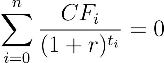
Unlike the Time-Weighted Rate of Return (TWRR), which neutralises the effect of external cash flows to isolate manager performance, MWRR reflects the investor's actual experienced return — incorporating the timing and magnitude of every deposit and withdrawal [3]. This makes it the metric of choice for client-facing reporting, personal rate of return statements, and scenarios where the investor controls the timing of cash flows.

Regulators, including bodies aligned with CFA Institute's Global Investment Performance Standards (GIPS), recognise both metrics but impose strict requirements on when each should be used, how they are calculated, and how they are disclosed [4]. Production systems must satisfy all of these constraints simultaneously — at scale, with auditability, and with deterministic behaviour.

2. The Computational Challenge: Solving a Polynomial with No Closed-Form Solution

2.1 Iterative Numerical Methods

MWRR requires finding the root of a high-degree polynomial. There is no closed-form algebraic solution [5]. Production systems must rely on iterative numerical methods, most commonly:

• Newton-Raphson Method — Fast convergence when the initial guess is close to the true root, but can diverge or oscillate if it is not [6].

• Secant Method — Does not require derivative computation, but shares many convergence risks with Newton-Raphson [6].

• Bisection Method — Guaranteed convergence if a valid bracket is known, but converges slowly [6].

• Brent's Method — A hybrid approach combining bisection with inverse quadratic interpolation, generally considered the most robust for production use [7].

The production implication: Every account, for every reporting period, requires running one of these solvers. There is no batch shortcut. Each solve is an independent numerical computation that must converge within acceptable tolerance and iteration limits. Your system must handle the case where it does not.

2.2 Multiple Roots

The MWRR polynomial is of degree n, where n corresponds to the number of distinct cash flow dates. By Descartes' Rule of Signs, the polynomial may have multiple positive real roots [8]. This occurs most commonly when:

• Cash flow directions alternate frequently (contributions followed by withdrawals followed by contributions).

• A large withdrawal exceeds the portfolio value at some intermediate point, creating a sign change in the effective "balance."

When multiple valid roots exist, the MWRR is mathematically ambiguous. There is no universally accepted convention for which root is "correct." Some vendors choose the root closest to zero; others choose the smallest positive root; others flag the result as indeterminate [9].

For auditors: If you are reviewing a system that returns a single MWRR value without disclosing whether multiple roots were detected, the result may be silently arbitrary. Your audit procedures should include test cases with alternating cash flows specifically designed to trigger multiple-root scenarios, and you should verify the system's documented selection policy.

2.3 No Real Root Exists

In certain degenerate cash flow patterns, no real root exists. This is mathematically possible when the polynomial has only complex roots for the given cash flow configuration [5]. Systems that do not handle this case will either:

• Return an incorrect value (the solver converges to a nonsensical number).

• Hang or time out (the solver runs to the maximum iteration count without convergence).

• Throw an unhandled exception.

Production requirement: A well-designed system must detect non-convergence, classify it, and surface it as a structured error — not a silent fallback to a default value.

3. Edge Cases That Break Naive Implementations

3.1 Zero or Near-Zero Starting Balances

When the beginning market value is zero (a new account funded during the period), the MWRR formula degenerates. The first cash flow effectively becomes the "investment," but the discount exponent depends on how intra-period timing is handled. Many implementations silently produce wildly incorrect annualised returns for accounts opened mid-period [10].

3.2 Very Short Periods

Computing MWRR over a single day or a handful of days, then annualising the result, amplifies noise to the point of absurdity. A 0.03% daily return becomes an annualised figure exceeding 11%. For periods under a threshold (commonly 1 year), production systems must decide: do they annualise or not? This is a business policy decision, but it has direct mathematical consequences and must be consistently applied and disclosed [4].

3.3 Large Cash Flows Relative to Portfolio Size

When a single cash flow is large relative to the portfolio value (e.g., a contribution that doubles the portfolio), MWRR becomes dominated by the return earned on that cash flow's timing. A contribution made the day before a market downturn produces a dramatically different MWRR than the same contribution made the day after [3]. This is mathematically correct — it is the intended behaviour of MWRR — but it creates client communication challenges and audit questions when the resulting return diverges significantly from the benchmark or from the TWRR.

3.4 Intraday Cash Flow Timing

MWRR formulas require a time fraction for each cash flow. Most implementations use a day-count convention (actual/365, actual/actual, or actual/360) [11]. But when does a cash flow "arrive" — at the start of the day, the end of the day, or at the exact timestamp of the transaction? The choice of convention (start-of-day, end-of-day, or mid-day weighting) measurably affects the computed return, particularly for large flows on volatile days. This convention must be documented, consistently applied, and available to auditors.

3.5 Trade Date vs. Settlement Date

A related issue: should cash flows be recorded on the trade date or the settlement date? The answer depends on the asset class, the client agreement, and the regulatory jurisdiction [12]. Production systems that serve multiple jurisdictions or asset classes may need to support both conventions simultaneously — per account, per asset class — and reconcile the difference.

4. Precision, Rounding, and Determinism

4.1 Floating-Point Arithmetic

Financial calculations demand precision. The IEEE 754 double-precision floating-point format carries approximately 15–17 significant decimal digits [13], which is generally sufficient for individual MWRR calculations. However, when aggregating returns across accounts, compounding over long periods, or comparing returns across systems, floating-point rounding errors accumulate.

Specific risk areas:

• Solver tolerance: The convergence tolerance of the iterative solver (e.g., |f(r)| < 1e-10) directly determines the precision of the output. A tolerance that is too loose produces inaccurate returns; one that is too tight causes unnecessary iterations or non-convergence.

• Day-count fractions: Dividing day counts produces repeating decimals (e.g., 1/3 of a year), introducing rounding at the exponent level.

• Compounding: Chaining sub-period MWRR values compounds rounding errors multiplicatively.

4.2 Determinism Across Platforms

A critical but often overlooked production concern: the same inputs must produce the same output regardless of the computing environment. Differences in floating-point implementations across CPU architectures (x86 vs. ARM), programming languages (strict vs. relaxed floating-point modes, native floats vs. arbitrary-precision decimals), and compiler optimisation levels can produce subtly different results [14]. For systems that must pass cross-platform reconciliation (e.g., a calculation engine producing results validated by an independent auditor's system), deterministic arithmetic is non-negotiable.

Recommendation for CTOs: Document the numerical methods, tolerances, and arithmetic standards used by your MWRR engine. Make these available to auditors as part of your methodology documentation. Consider using arbitrary-precision decimal arithmetic for the final rounding step, even if the iterative solver uses floating-point internally.

5. Performance at Scale

5.1 The Computational Cost

Each MWRR computation requires an iterative solve. For a typical portfolio with monthly cash flows over 10 years, the solver must find the root of a polynomial with ~120 terms. Newton-Raphson typically converges in 10–30 iterations; Brent's method may require 40–60 [7].

Now multiply by the number of accounts. A wealth management platform serving 500,000 clients, each with 3–5 accounts, computing daily MWRR for trailing 1-month, 3-month, YTD, 1-year, 3-year, 5-year, and since-inception periods, is executing on the order of tens of millions of independent solver invocations per day. Each invocation is inherently sequential (the next iteration depends on the previous), limiting parallelisation within a single solve.

5.2 Strategies for Production Throughput

• Parallelisation across accounts: Each account's MWRR is independent. The workload is embarrassingly parallel at the account level [15]. Systems should be designed around this property.

• Caching and incremental computation: For rolling periods, much of the cash flow data is unchanged from the previous day. Intelligent caching of intermediate results can reduce redundant computation, though the non-linear nature of MWRR limits the effectiveness of simple memoisation.

• Tiered computation: Not all periods need to be recomputed daily. Since-inception returns for stable, low-activity accounts can be recomputed weekly or on-demand, while YTD and trailing-month returns are computed nightly.

• Solver warm-starting: Using the previous day's MWRR as the initial guess for today's solve dramatically improves convergence speed, since returns rarely change drastically day-over-day.

5.3 Timeout and Circuit-Breaker Policies

Production systems must enforce maximum iteration counts and wall-clock timeouts per computation. A single pathological account (with complex cash flow patterns causing non-convergence) should not block the batch. Implement circuit breakers [16]: if a computation exceeds limits, log it, flag the account for manual review, and continue processing the rest of the batch.

6. Auditability and Reconciliation

6.1 Why MWRR is Hard to Audit

TWRR is relatively straightforward to audit: you can independently verify each sub-period return and confirm the geometric linking [3]. MWRR, by contrast, is an opaque function — you feed in cash flows and get a single rate out of an iterative solver. There is no intermediate decomposition to inspect.

This creates a significant auditability gap. An auditor cannot easily:

• Verify partial results (there are none — the solver produces a single output).

• Attribute return to sub-periods (MWRR is not decomposable).

• Manually recalculate without access to the same solver implementation.

6.2 Audit Recommendations

For auditors:

1. Demand methodology documentation. The system's numerical method, convergence tolerance, maximum iterations, initial guess strategy, multiple-root handling policy, day-count convention, and cash flow timing convention must all be documented.

2. Use independent solver implementations. Recalculate a sample of accounts using a different solver (even a spreadsheet-based IRR function [17]) and verify results match within stated tolerance.

3. Test boundary conditions explicitly. Provide the system with test cases designed to trigger edge cases: zero starting balance, single-day periods, alternating cash flows, and extremely large relative cash flows. Verify behaviour matches documented policy.

4. Verify consistency over time. Recalculate a historical period's MWRR using today's system and confirm it matches the originally reported value. Changes in methodology, tolerance, or convention should be versioned and disclosed.

5. Inspect non-convergence handling. Request the system's log of accounts where the solver did not converge. Verify these were flagged, not silently defaulted.

6.3 Reproducibility

A production MWRR engine must be able to reproduce any previously computed return given the same inputs. This requires:

• Immutable cash flow records: Cash flows must be versioned. Retroactive corrections (e.g., a contribution backdated to last month) must produce a new version of the return, not silently overwrite the previous one [18].

• Methodology versioning: If the solver tolerance, day-count convention, or any other parameter changes, the system must record which version of the methodology was in effect for each computation.

• Input snapshotting: The market values and cash flows used for each computation should be retrievable. Without this, reproduction is impossible.

7. Regulatory and Compliance Considerations

7.1 GIPS Standards

The CFA Institute's Global Investment Performance Standards (GIPS®) require money-weighted returns for certain composites, particularly in private equity and real estate, where cash flows are not under the manager's control [4]. GIPS mandates:

• Minimum frequency of return calculation.

• Specific annualization rules (returns for periods of less than one year must not be annualised) [4].

• Disclosure requirements when approximations are used.

Production systems serving GIPS-compliant firms must enforce these rules programmatically, not rely on manual oversight.

7.2 MiFID II and Client Reporting

Under MiFID II, investment firms must provide clients with performance reports that include costs and charges [19]. When MWRR is used for personal rate of return, the methodology must be disclosed to the client, and the return must reflect the actual impact of costs. This means fee cash flows must be correctly classified and included in the MWRR computation.

7.3 SEC and FINRA Considerations

In the U.S., SEC Marketing Rule (Rule 206(4)-1 under the Investment Advisers Act) and FINRA advertising rules have specific requirements about which return methodology can be used in marketing materials versus client statements [20] [21]. Using MWRR where TWRR is required (or vice versa) is a compliance violation. Production systems must enforce the correct methodology per context.

8. Operational Risks and Failure Modes

9. Recommendations for CTOs

1. Treat MWRR as a numerical computing problem, not a simple formula. Staff the team with engineers who understand numerical methods, convergence analysis, and floating-point arithmetic — or use a well-tested, well-documented numerical computing library with proven root-finding implementations.

2. Invest in observability. Log every computation: inputs, outputs, iterations to convergence, whether multiple roots were detected, and whether the result was flagged. This is your audit trail.

3. Design for failure. Every MWRR computation can fail. Your architecture must handle non-convergence, multiple roots, and edge cases gracefully — with structured errors, not silent defaults. Consider adopting resilience patterns from distributed systems literature [16].

4. Version your methodology. Any change to solver parameters, day-count conventions, cash flow timing, or rounding rules must be versioned, dated, and traceable. Auditors will ask for this.

5. Benchmark your solver. Maintain a suite of test cases — including adversarial ones — and run them as part of your CI/CD pipeline. Regression in a financial calculation is a regulatory event, not just a bug.

6. Separate computation from presentation. Store MWRR at full solver precision. Apply rounding only at the presentation layer. This preserves the ability to reconcile and recompute without introducing additional rounding error.

7. Consider TWRR as a complement, not a replacement. Many production systems compute both MWRR and TWRR, using the divergence between them as a diagnostic signal [3]. A large MWRR-TWRR gap indicates a significant cash flow timing impact, which may warrant client communication or additional disclosure.

10. Conclusion

MWRR is a deceptively simple concept with production implications that span numerical computing, systems architecture, regulatory compliance, and audit readiness. The challenges are not theoretical — they manifest as incorrect client statements, failed audits, compliance violations, and operational incidents.

For CTOs, the path forward is clear: treat the MWRR engine as critical financial infrastructure, subject to the same rigour as trade execution or settlement systems. For auditors, the imperative is equally clear: do not accept MWRR as a black box. Demand methodology documentation, test boundary conditions, and verify reproducibility.

The organisations that get this right build trust with clients and regulators alike. Those that don't discover the consequences in production, where the cost of a wrong number is measured not in basis points, but in reputation.

References

[1] Brealey, R. A., Myers, S. C., & Allen, F. (2020). Principles of Corporate Finance (13th ed.). McGraw-Hill Education. — Establishes the mathematical equivalence between IRR and money-weighted returns.

[2] Maginn, J. L., Tuttle, D. L., Pinto, J. E., & McLeavey, D. W. (2007). Managing Investment Portfolios: A Dynamic Process (3rd ed.). CFA Institute Investment Series, John Wiley & Sons. — Provides the formal NPV-based definition of money-weighted rate of return.

[3] Bacon, C. R. (2023). Practical Portfolio Performance Measurement and Attribution (3rd ed.). John Wiley & Sons. — The definitive reference on the distinction between MWRR and TWRR, including practical implications of cash flow timing on return divergence.

[4] CFA Institute. (2020). Global Investment Performance Standards (GIPS®) for Firms. CFA Institute. Available at: https://www.gipsstandards.org — The authoritative standard governing investment performance reporting, including MWRR requirements for private equity and real estate composites.

[5] Hazen, G. B. (2003). "A New Perspective on Multiple Internal Rates of Return." The Engineering Economist, 48(1), 31–51. DOI: 10.1080/00137910308965050 — Analyzes the conditions under which multiple IRR solutions exist and the implications for financial decision-making.

[6] Press, W. H., Teukolsky, S. A., Vetterling, W. T., & Flannery, B. P. (2007). Numerical Recipes: The Art of Scientific Computing (3rd ed.). Cambridge University Press. — Comprehensive reference on iterative root-finding methods including Newton-Raphson, Secant, and Bisection.

[7] Brent, R. P. (1973). Algorithms for Minimization Without Derivatives. Prentice-Hall. Reprinted by Dover Publications, 2002. — The original description of Brent's method, widely regarded as the most robust general-purpose root-finding algorithm.

[8] Loy, J. (2001). "Descartes' Rule of Signs." Mathematics Magazine. — Reference on the application of Descartes' Rule of Signs to polynomial root counting, applicable to IRR polynomials.

[9] Osborne, M. J. (2010). "A Resolution to the NPV–IRR Debate?" The Quarterly Review of Economics and Finance, 50(2), 234–239. DOI: 10.1016/j.qref.2010.01.002 — Discusses the ambiguity of multiple IRR solutions and proposed resolution methods.

[10] Spaulding, D. (2003). Investment Performance Measurement. McGraw-Hill. — Covers practical implementation pitfalls in performance measurement, including handling of accounts with zero starting balances.

[11] International Swaps and Derivatives Association (ISDA). (2006). 2006 ISDA Definitions. ISDA. Available at: https://www.isda.org — Industry standard reference for day-count conventions (Actual/365, Actual/360, Actual/Actual, 30/360).

[12] Securities Industry and Financial Markets Association (SIFMA). "Standard Settlement Cycles." Available at: https://www.sifma.org — Documents settlement conventions across asset classes and jurisdictions, relevant to trade date vs. settlement date decisions.

[13] IEEE Computer Society. (2019). IEEE Standard for Floating-Point Arithmetic (IEEE 754-2019). IEEE. DOI: 10.1109/IEEESTD.2019.8766229 — The authoritative specification for floating-point arithmetic, governing precision and rounding behavior.

[14] Goldberg, D. (1991). "What Every Computer Scientist Should Know About Floating-Point Arithmetic." ACM Computing Surveys, 23(1), 5–48. DOI: 10.1145/103162.103163 — Seminal paper on floating-point arithmetic pitfalls, essential reading for engineers building financial calculation systems.

[15] Herlihy, M. & Shavit, N. (2012). The Art of Multiprocessor Programming (Revised 1st ed.). Morgan Kaufmann. — Reference on parallelization strategies applicable to embarrassingly parallel workloads like per-account return computation.

[16] Nygard, M. T. (2018). Release It! Design and Deploy Production-Ready Software (2nd ed.). Pragmatic Bookshelf. — Describes circuit breaker patterns and resilience strategies for production systems handling computationally intensive workloads.

[17] Shestopaloff, Y. K. (2009). "Properties and Interrelationships of Polynomial, Exponential, and Hyperbolic Money-Weighted Rates of Return." Journal of Performance Measurement, 13(3), 38–52. — Analyzes different formulations of money-weighted returns and the use of spreadsheet-based IRR functions as independent verification tools.

[18] Kleppmann, M. (2017). Designing Data-Intensive Applications. O'Reilly Media. — Provides foundational concepts for immutable data architecture and event sourcing, applicable to versioned cash flow record keeping.

[19] European Securities and Markets Authority (ESMA). (2018). MiFID II — Guidelines on Costs and Charges Disclosure. ESMA. Available at: https://www.esma.europa.eu — Regulatory guidance on cost disclosure in client performance reports under MiFID II.

[20] U.S. Securities and Exchange Commission. (2020). Investment Adviser Marketing Rule (Rule 206(4)-1). SEC. Available at: https://www.sec.gov/rules/final/2020/ia-5653.pdf — SEC rule governing the use of performance metrics in investment adviser marketing materials.

[21] Financial Industry Regulatory Authority (FINRA). FINRA Rule 2210 — Communications with the Public. FINRA. Available at: https://www.finra.org/rules-guidance/rulebooks/finra-rules/2210 — FINRA rules on the presentation of performance data in communications with retail investors.

Disclaimer: This article is intended for informational purposes and does not constitute financial, legal, or regulatory advice. Organisations should consult with qualified professionals when designing performance measurement systems or audit procedures.